Hypothesis testing
Hypothesis testing
When interpreting research findings, researchers need to assess whether these findings may have occurred by chance. Hypothesis testing is a systematic procedure for deciding whether the results of a research study support a particular theory which applies to a population.
Hypothesis testing uses sample data to evaluate a hypothesis about a population. A hypothesis test assesses how unusual the result is, whether it is reasonable chance variation or whether the result is too extreme to be considered chance variation.
Basic concepts
Null and research hypotheses
To carry out statistical hypothesis testing, research and null hypothesis are employed:
- Research hypothesis: this is the hypothesis that you propose, also known as the alternative hypothesis HA. For example:
HA: There is a relationship between intelligence and academic results.
HA: First year university students obtain higher grades after an intensive Statistics course.
HA; Males and females differ in their levels of stress.
- The null hypothesis (Ho) is the opposite of the research hypothesis and expresses that there is no relationship between variables, or no differences between groups; for example:
Ho: There is no relationship between intelligence and academic results.
Ho: First year university students do not obtain higher grades after an intensive Statistics course.
Ho: Males and females will not differ in their levels of stress.
The purpose of hypothesis testing is to test whether the null hypothesis (there is no difference, no effect) can be rejected or approved. If the null hypothesis is rejected, then the research hypothesis can be accepted. If the null hypothesis is accepted, then the research hypothesis is rejected.
In hypothesis testing, a value is set to assess whether the null hypothesis is accepted or rejected and whether the result is statistically significant:
- A critical value is the score the sample would need to decide against the null hypothesis.
- A probability value is used to assess the significance of the statistical test. If the null hypothesis is rejected, then the alternative to the null hypothesis is accepted.
Probability value and types of errors
The probability value, or p value, is the probability of an outcome or research result given the hypothesis. Usually, the probability value is set at 0.05: the null hypothesis will be rejected if the probability value of the statistical test is less than 0.05. There are two types of errors associated to hypothesis testing:
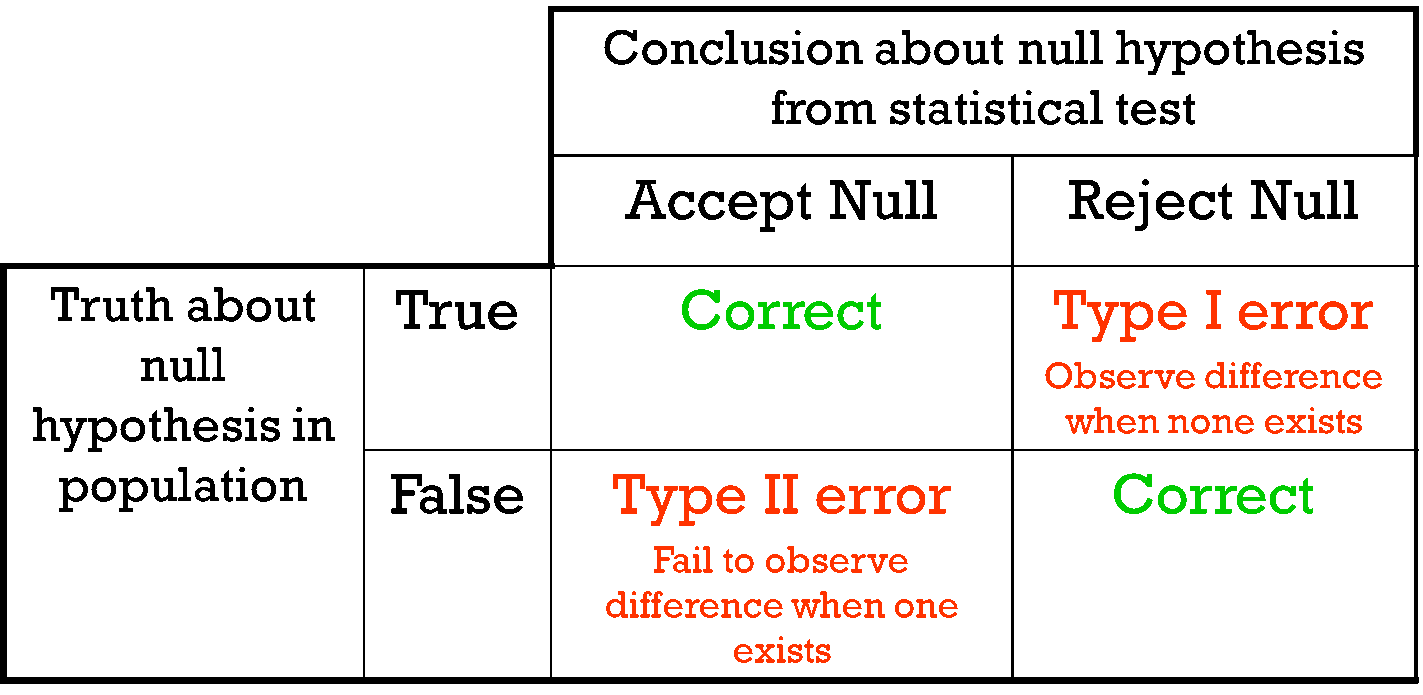
- What if we observe a difference – but none exists in the population?
- What if we do not find a difference – but it does exist in the population?
These situations are known as Type I and Type II errors:
- Type I Error: is the type of error that involves the rejection of a null hypothesis that is actually true (i.e. a false positive).
- Type II Error: is the type of error that occurs when we do not reject a null hypothesis that is false (i.e. a false negative).
These errors cannot be eliminated; they can be minimised, but minimising one type of error will increase the probability of committing the other type.
The probability of making a Type I error depends on the criterion that is used to accept or reject the null hypothesis: the p value or alpha level. The alpha is set by the researcher, usually at .05, and is the chance the researcher is willing to take and still claim the significance of the statistical test.). Choosing a smaller alpha level will decrease the likelihood of committing Type I error.
For example, p<0.05 indicates that there are 5 chances in 100 that the difference observed was really due to sampling error – that 5% of the time a Type I error will occur or that there is a 5% chance that the opposite of the null hypothesis is actually true.
With a p<0.01, there will be 1 chance in 100 that the difference observed was really due to sampling error – 1% of the time a Type I error will occur.
The p level is specified before analysing the data. If the data analysis results in a probability value below the α (alpha) level, then the null hypothesis is rejected; if it is not, then the null hypothesis is not rejected.
Effect size and statistical significance
When the null hypothesis is rejected, the effect is said to be statistically significant. However, statistical significance does not mean that the effect is important.
A result can be statistically significant, but the effect size may be small. Finding that an effect is significant does not provide information about how large or important the effect is. In fact, a small effect can be statistically significant if the sample size is large enough.
Information about the effect size, or magnitude of the result, is given by the statistical test. For example, the strength of the correlation between two variables is given by the coefficient of correlation, which varies from 0 to 1.
- A directional hypothesis specifies the direction of the relationship between independent and dependent variables.
- A hypothesis that states that students who attend an intensive Statistics course will obtain higher grades than students who do not attend would be directional.
- A non-directional hypothesis states that there will be a difference, but we do not know what direction that will be.
- A non-directional hypothesis states that there will be differences between students who attend do or don’t attend an intensive Statistics course, but we don’t know what group will get higher grades than the other. The hypothesis only states that they will obtain different grades.
The hypothesis testing process
The hypothesis testing process can be divided into five steps:
- Restate the research question as research hypothesis and a null hypothesis about the populations.
- Determine the characteristics of the comparison distribution.
- Determine the cut off sample score on the comparison distribution at which the null hypothesis should be rejected.
- Determine your sample’s score on the comparison distribution.
- Decide whether to reject the null hypothesis.
This example illustrates how these five steps can be applied to text a hypothesis:
- Let’s say that you conduct an experiment to investigate whether students’ ability to memorise words improves after they have consumed caffeine.
- The experiment involves two groups of students: the first group consumes caffeine; the second group drinks water.
- Both groups complete a memory test.
- A randomly selected individual in the experimental condition (i.e. the group that consumes caffeine) has a score of 27 on the memory test. The scores of people in general on this memory measure are normally distributed with a mean of 19 and a standard deviation of 4.
- The researcher predicts an effect (differences in memory for these groups) but does not predict a particular direction of effect (i.e. which group will have higher scores on the memory test). Using the 5% significance level, what should you conclude?
Step 1: There are two populations of interest.
Population 1: People who go through the experimental procedure (drink coffee).
Population 2: People who do not go through the experimental procedure (drink water).
- Research hypothesis: Population 1 will score differently from Population 2.
- Null hypothesis: There will be no difference between the two populations.
Step 2: We know that the characteristics of the comparison distribution (student population) are:
Population M = 19, Population SD= 4, normally distributed. These are the mean and standard deviation of the distribution of scores on the memory test for the general student population.
Step 3: For a two-tailed test (the direction of the effect is not specified) at the 5% level (25% at each tail), the cut off sample scores are +1.96 and -1.99.
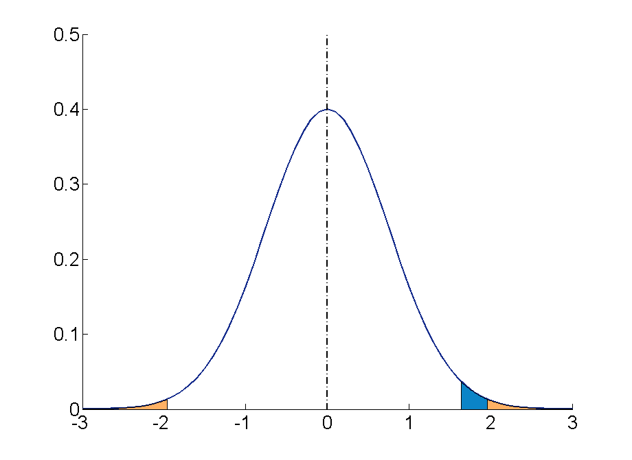
Step 4: Your sample score of 27 needs to be converted into a Z value. To calculate Z = (27-19)/4= 2 (check the Converting into Z scores section if you need to review how to do this process)
Step 5: A ‘Z’ score of 2 is more extreme than the cut off Z of +1.96 (see figure above). The result is significant and, thus, the null hypothesis is rejected.
You can find more examples here:
Some commonly used statistical techniques
Correlation analysis
Correlation analysis explores the association between variables. The purpose of correlational analysis is to discover whether there is a relationship between variables, which is unlikely to occur by sampling error. The null hypothesis is that there is no relationship between the two variables. Correlation analysis provides information about:
- The direction of the relationship: positive or negative- given by the sign of the correlation coefficient.
- The strength or magnitude of the relationship between the two variables- given by the correlation coefficient, which varies from 0 (no relationship between the variables) to 1 (perfect relationship between the variables).
- Direction of the relationship.
A positive correlation indicates that high scores on one variable are associated with high scores on the other variable; low scores on one variable are associated with low scores on the second variable . For instance, in the figure below, higher scores on negative affect are associated with higher scores on perceived stress

A negative correlation indicates that high scores on one variable are associated with low scores on the other variable. The graph shows that a person who scores high on perceived stress will probably score low on mastery. The slope of the graph is downwards- as it moves to the right. In the figure below, higher scores on mastery are associated with lower scores on perceived stress.
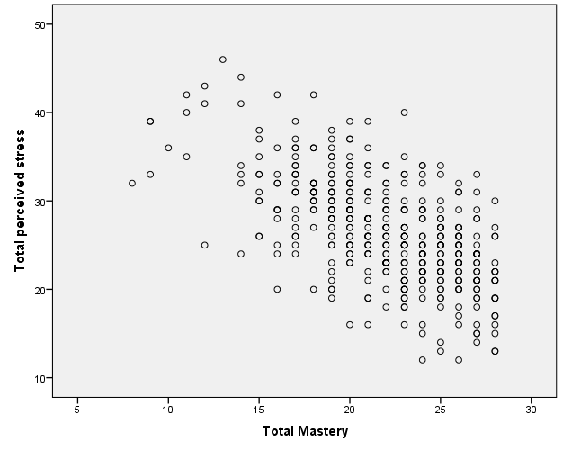
Fig 2. Negative correlation between two variables. Adapted from Pallant, J. (2013). SPSS survival manual: A step by step guide to data analysis using IBM SPSS (5th ed.). Sydney, Melbourne, Auckland, London: Allen & Unwin
2. The strength or magnitude of the relationship
The strength of a linear relationship between two variables is measured by a statistic known as the correlation coefficient, which varies from 0 to -1, and from 0 to +1. There are several correlation coefficients; the most widely used are Pearson’s r and Spearman’s rho. The strength of the relationship is interpreted as follows:
- Small/weak: r= .10 to .29
- Medium/moderate: r= .30 to .49
- Large/strong: r= .50 to 1
It is important to note that correlation analysis does not imply causality. Correlation is used to explore the association between variables, however, it does not indicate that one variable causes the other. The correlation between two variables could be due to the fact that a third variable is affecting the two variables.
Multiple regression
Multiple regression is an extension of correlation analysis. Multiple regression is used to explore the relationship between one dependent variable and a number of independent variables or predictors. The purpose of a multiple regression model is to predict values of a dependent variable based on the values of the independent variables or predictors. For example, a researcher may be interested in predicting students’ academic success (e.g. grades) based on a number of predictors, for example, hours spent studying, satisfaction with studies, relationships with peers and lecturers.
A multiple regression model can be conducted using statistical software (e.g. SPSS). The software will test the significance of the model (i.e. does the model significantly predicts scores on the dependent variable using the independent variables introduced in the model?), how much of the variance in the dependent variable is explained by the model, and the individual contribution of each independent variable.
Example of multiple regression model
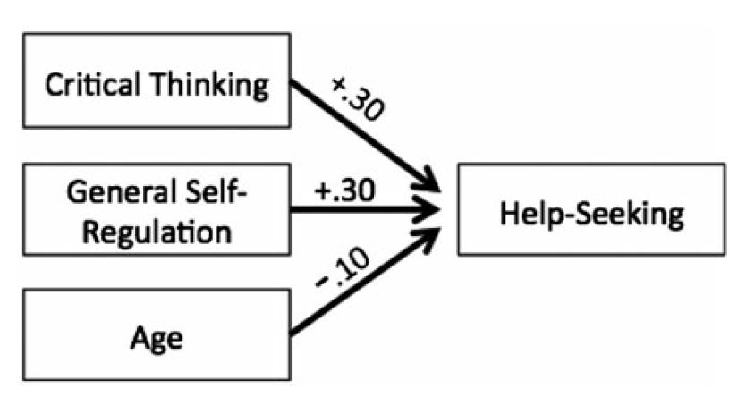
From Dunn et al. (2014). Influence of academic self-regulation, critical thinking, and age on online graduate students' academic help-seeking.
In this model, help-seeking is the dependent variable; there are three independent variables or predictors. The coefficients show the direction (positive or negative) and magnitude of the relationship between each predictor and the dependent variable. The model was statistically significant and predicted 13.5% of the variance in help-seeking.
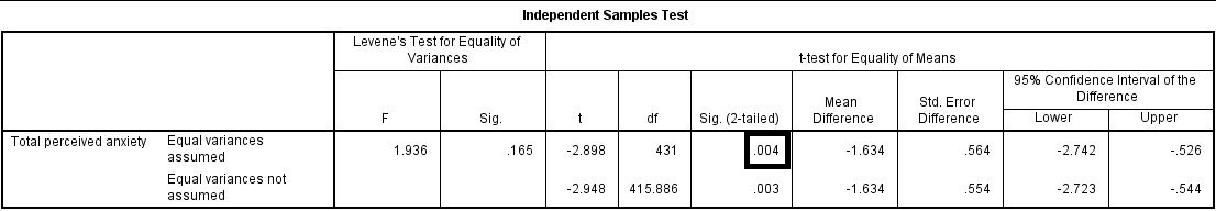
t-Tests
t-Tests are employed to compare the mean score on some continuous variable for two groups. The null hypothesis to be tested is there are no differences between the two groups (e.g. anxiety scores for males and females are not different).
If the significance value of the t-test is equal or less than .05, there is a significant difference in the mean scores on the variable of interest for each of the two groups. If the value is above .05, there is no significant difference between the groups.
t-Tests can be employed to compare the mean scores of two different groups (independent-samples t-test) or to compare the same group of people on two different occasions (paired-samples t-test).
In addition to assessing whether the difference between the two groups is statistically significant, it is important to consider the effect size or magnitude of the difference between the groups. The effect size is given by partial eta squared (proportion of variance of the dependent variable that is explained by the independent variable) and Cohen’s d (difference between groups in terms of standard deviation units).
In this example, an independent samples t-test was conducted to assess whether males and females differ in their perceived anxiety levels. The significance of the test is .004. Since this value is less than .05, we can conclude that there is a statistically significant difference between males and females in their perceived anxiety levels.
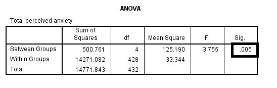
ANOVA
Whilst t-tests compare the mean score on one variable for two groups, analysis of variance is used to test more than two groups. Following the previous example, analysis of variance would be employed to test whether there are differences in anxiety scores for students from different disciplines.
Analysis of variance compare the variance (variability in scores) between the different groups (believed to be due to the independent variable) with the variability within each group (believed to be due to chance). An F ratio is calculated; a large F ratio indicates that there is more variability between the groups (caused by the independent variable) than there is within each group (error term). A significant F test indicates that we can reject the null hypothesis; i.e. that there is no difference between the groups.
Again, effect size statistics such as Cohen’s d and eta squared are employed to assess the magnitude of the differences between groups.
In this example, we examined differences in perceived anxiety between students from different disciplines. The results of the Anova Test show that the significance level is .005. Since this value is below .05, we can conclude that there are statistically significant differences between students from different disciplines in their perceived anxiety levels.
Chi-square test for independence
Chi-square test for independence is used to explore the relationship between two categorical variables. Each variable can have two or more categories.
For example, a researcher can use a Chi-square test for independence to assess the relationship between study disciplines (e.g. Psychology, Business, Education,…) and help-seeking behaviour (Yes/No). The test compares the observed frequencies of cases with the values that would be expected if there was no association between the two variables of interest. A statistically significant Chi-square test indicates that the two variables are associated (e.g. Psychology students are more likely to seek help than Business students). The effect size is assessed using effect size statistics: Phi and Cramer’s V.
In this example, a Chi-square test was conducted to assess whether males and females differ in their help-seeking behaviour (Yes/No). The crosstabulation table shows the percentage of males of females who sought/didn't seek help. The table 'Chi square tests' shows the significance of the test (Pearson Chi square asymp sig: .482). Since this value is above .05, we conclude that there is no statistically significant difference between males and females in their help-seeking behaviour.
