Measures of variability
Descriptive statistics: measures of variability
Variability refers to how spread scores are in a distribution out; that is, it refers to the amount of spread of the scores around the mean. For example, distributions with the same mean can have different amounts of variability or dispersion.
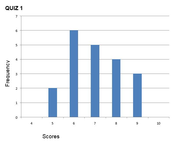
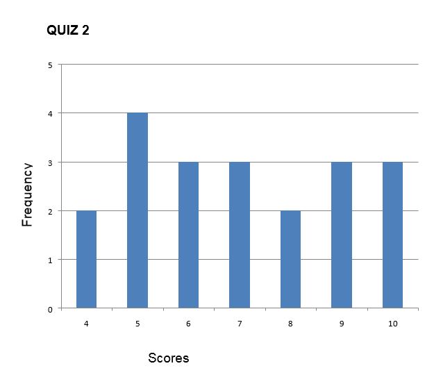
In the following two histograms, the distribution of scores for Quiz 1 and Quiz 2 are presented. Despite the equal means (the mean score for both quizzes is 7), the scores on Quiz 1 are more packed or clustered around the mean, whilst the scores on Quiz 2 are more spread out. Thus, the differences within the student group were greater on Quiz 2 than on Quiz 1.
There are four frequently used measures of the variability of a distribution:
- range
- interquartile range
- variance
- standard deviation.
Measures of variability
Range
The most basic measure of variation is the range, which is the distance from the smallest to the largest value in a distribution.
Range= Largest value – Smallest Value
For the distribution of scores of Quiz 1 and Quiz 2, the range is:
Quiz 1. Range = 9-5= 4
Quiz 2. Range = 10-4= 6
which shows (like the histograms above) that Quiz 2 scores have greater spread than Quiz 1 scores.
However, the range uses only two values in the data set, and one of these values may be an unusually large or small value.
Interquartile range
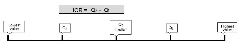
The interquartile range (IQR) is the range of the middle 50% scores in a distribution:
IQR= 75th percentile – 25th percentile
It is based on dividing a data set into quartiles. Quartiles are the values that divide scores into quarters. Q1 is the lower quartile and is the middle number between the smallest number and the median of a data set. Q2 is the middle quartile-or median. Q3 is the upper quartile and is the middle value between the median set and the highest value of a data set. The interquartile range formula is the first quartile subtracted from the third quartile
For Quiz 1, Q3 is 8 and Q1 is 6 . These are the scores:
5, 6, 7, 8, 9
If the median is 7, then Q1 is 6 (middle value between median and lowest value) and Q3 is 8 (middle value between median and highest value).
To calculate the IQR:
IQR= 8-6= 2
For Quiz 2, Q3 is 9 and Q1 is 5. These are the scores:
4, 5, 6, 7, 8, 9, 10
The median is 7. To find Q1, we’ll look at the lower half section of the distribution of scores: 4,5,6. Q 1 is the median of this section of the distribution: 5
To find Q2, we’ll look at the upper half section of the distribution of scores: 8, 9,10. Q3 is the median of this section of the distribution: 9.
To calculate the IQR, knowing Q1 and Q3:
IQR= 9-5= 4
Variance
The variance is the average squared difference of the scores from the mean. To compute the variance in a population:
- Calculate the mean
- Subtract the mean from each score to compute the deviation from mean score
- Square each deviation score (multiply each score by itself)
- Add up the squared deviation score to give the sum
- Divide the sum by the number of scores
The table below contains students’ scores on a Statistics test. To calculate the variance:
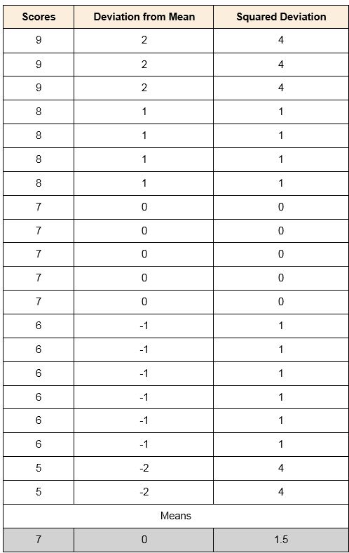
- The mean is calculated: sum all scores and divide by the number of scores: 140/20= 7
- The deviation from the mean for each score is calculated. For example, for the first score: 9-7= 2- See column Deviation from the mean
- Each deviation from the mean score is squared (multiplied by itself). For the first score: 2x2= 4. See column Squared deviation.
- Finally, the mean of the squared deviations is calculated. The variance is 1.5
This is how the formula to calculate variance in a population looks like:

Where o2 is the variance
µ is the mean of a population
X are the values or scores
N is the number of values or scores
If the variance in a sample is used to estimate the variance in a population, it is important to note that samples are consistently less variable than their populations:
- The sample variability gives a biased estimate of the population variability.
- This bias is in the direction of underestimating the population value.
- In order to adjust this consistent underestimation of the population variance, we divide the sum of the squared deviation by N-1 instead of N.
Formula to calculate variance in a sample is:

Where s2 is the variance of the sample
M is the sample mean
X are the values or scores
N is the number of values or scores in the sample
Standard deviation
The standard deviation is the average amount by which scores differ from the mean. The standard deviation is the square root of the variance, and it is a useful measure of variability when the distribution is normal or approximately normal (see below on the normality of distributions). The proportion of the distribution within a given number of standard deviations (or distance) from the mean can be calculated.
A small standard deviation coefficient indicates a small degree of variability (that is, scores are close together); larger standard deviation coefficients indicate large variability (that is, scores are far apart).
The formula to calculate the standard deviation is

Note that the standard deviation is the square root of the variance.
Example: how to calculate the standard deviation:
In the previous section- Variance- we computed the variance of scores on a Statistics test by calculating the distance from the mean for each score,t hen squaring each deviation from the mean, and finally calculating the mean of the squared deviations.
Since we already know the variance, we can use it to calculate the standard deviation. To do so, take the square root of the variance. The square root of 1.5 is 1.22. The standard deviation is 1.22.
Distributions with the same mean can have different standard deviations. As mentioned before, a small standard deviation coefficient indicates that scores are close together, whilst a large standard deviation coefficient indicates that scores are far apart. In this example, both sets of data have the same mean, but the standard deviation coefficient is different:

In this example, the scores in Set A are 0.82 away from the mean; in Set B, scores are 2.65 away from the mean, even though the mean is the same for both sets. So scores in Set B are more dispersed than scores in Set A.
Activity 1: Mean and standard deviation
Shapes of distributions: skewness and kurtosis
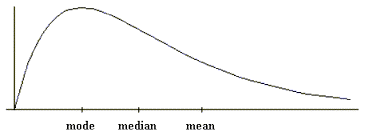
Distributions can be asymmetrical or skewed; that is, the tail of the distribution in the positive direction extends further than the tail in the negative direction, or vice versa. A distribution with the longer tail extending in the positive direction is said to have a positive skew; it is skewed to the right.
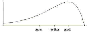
A distribution with the longer tail extending to the left is negatively skewed, or skewed to the left:
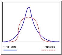
Distributions also differ in terms of whether the data are peaked or flat. Distributions with positive kurtosis have a distinct peak near the mean and decline rapidly, whilst distributions with negative kurtosis tend to be more flat:
Normal distributions
The normal distribution is the most important and commonly used distribution in statistics. It is also known as the bell curve or Gaussian curve. Even though normal distributions can differ in their means and standard deviation, they share some characteristics related to the distribution of scores:
- they are symmetric around their mean
- the mean, median, and mode are equal
- are denser in the center and less dense in the tails
- are defined by two parameters: the mean and standard deviation
- 68% of the area is within one standard deviation of the mean
- approximately 95% of the area is within two standard deviations of the mean
- 99.7 % of the area is within 3 standard deviations of the mean.
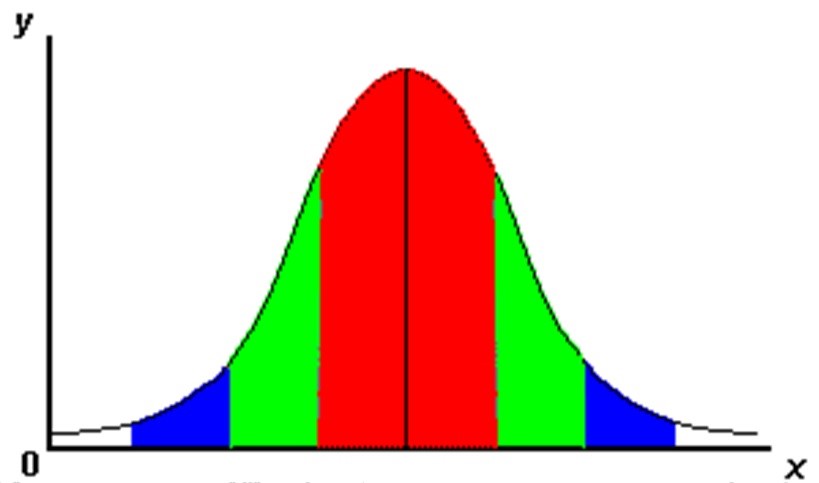
The 68-95-99.7% rule
Standard normal deviations follow the 68-95-99.7% rule:
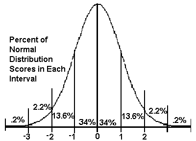
- 68% of scores are within one standard deviation of the mean.
- 95% of scores are within 2 standard deviations of the mean.
- 99.7% of scores are within 3 standard deviations of the mean.
Knowing the mean and standard deviation of a normal distribution, we can calculate the values that lie within 1 standard deviation of the mean.
For example, if the mean of a normal distribution is 25 years (age) and the standard distribution is 8 years, then:
- 68% of people will be between 17 (25-8= 17) and 33 years ( 25+8= 33).
Statistical symbols used in this page
o2- variance in a population
µ- mean of a population
M- mean of a sample
s2- variance in a sample